Methods for analysis of spatial peptidergic communication networks
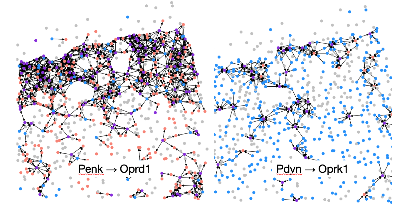
Communication in the brain can occur between cells that release specific neuropeptides and cells that sense these neuropeptides. In this study, we develop computational methods to study the organization of this form of communication. We explore regimes in which neighborhood information is helpful for cell type classification with graph neural networks and adapt Node2Vec (Grover and Leskovec 2016) to obtain multilayer graph embeddings.
Background on neuropeptidergic communication
We study neuropeptidergic communication between ligands and receptors in the brain. Ligands are small molecules that bind selectively to receptor proteins. The ligands of interest are peptides (small chains of amino acids), and the receptor proteins of interest are G-protein coupled receptors or GPCRs (Rosenbaum, Rasmussen, and Kobilka 2009). Peptides released by one neuron can bind to GPCRs on other neurons and modulate their activity. Many such cognate neuropeptide-GPCR pairs have been identified in the literature.
Single cell transcriptomic data suggests that a vast majority of cortical neurons participate in such communication in a cell-type dependent manner (Smith et al. 2019). Thus, compatible (a.k.a cognate) peptide-GPCR pairs can be considered as an unique communication channel between neurons (Smith et al. 2019).
It is important to study these networks because combinatorial expression of neuropeptides and receptors enables local, type specific communication between neurons. Such peptidergic signaling is slower and longer lasting compared to synaptic signaling. Computational studies also suggest that such neuron-type–specific local neuromodulation may be a critical piece of the biological credit-assignment puzzle (Liu et al. 2021).
Background on spatial transcriptomic data
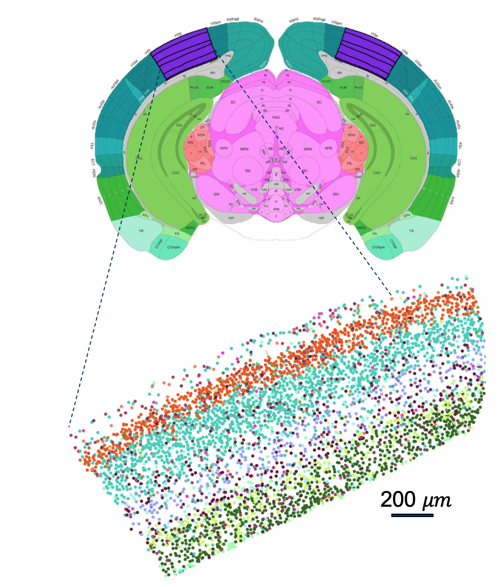
We study spatial peptidergic communication networks with spatial transcriptomic data. Spatial transcriptomic experiments measure gene expression while preserving spatial context. There are many technologies to acquire such data, with trade-offs in spatial resolution, speed, and compatibility with other kinds of experiments on the same tissue sample Chen et al. (2023). Some of these technologies, namely SeqFISH, MERFISH, Slide-Seq have been used to produce atlas scale datasets in the mouse brain by the BICCN (Hawrylycz et al. 2023). We consider a recent whole mouse brain dataset obtained with an in-situ hybridization-based technique called MERFISH (Yao et al. 2023). This dataset consists of expression measurements of approximately 500 genes in 4 million cells from a single mouse brain. We focus on the primary visual cortex (VISp region) in this study as shown in Figure 2.
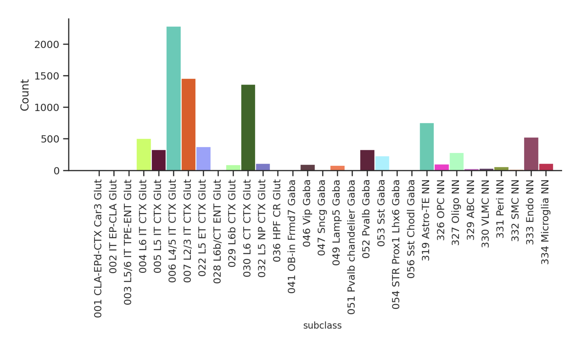
We note that the subclass distribution of cells in the dataset is imbalanced. This makes subclass classification tasks more difficult.
Neuropeptidergic communication as directed multilayer graphs
Peptidergic communication networks can be viewed as directed multilayer graphs.
The multilayer graph G is the set \(\{V, \{E_l\}\}\) where:
\(V\) is the set of vertices (cells).
\(E_l\) s the set of directed edges for the lth network.
For the \(l\) th network, an edge exists from vertex \(i\) to vertex \(j\) if all the following conditions are met:
- distance \(d[i,j] \leq d_{threshold}\)
- vertex i expresses the peptide precursor gene
- vertex j expresses the GPCR gene
The peptidergic multilayer graph does not contain any edges between layers. We set \(d_{threshold} = 40 \textmu m\) for all experiments unless mentioned otherwise.
Code for graph construction can be found here.

5 neuropeptide precursor and GPCR pairs were experimentally measured in the MERFISH dataset. The 5 pairs each make up a layer in the multilayer graph as shown in Figure 4.
Node classification with graph neural networks
We first explore regimes in which neighborhood information is helpful for cell type classification with graph neural networks. Graph neural networks combine features of nodes that are adjacent according to the underlying graph.
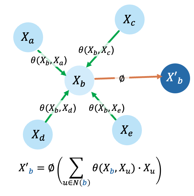
A nonlinear function ∅ of aggregated (sum here) weighted node features determines updated node representation. In GATv2, the node features are weighted using a function of node pairs, \(\theta\) (Brody, Alon, and Yahav 2021). Functions \(\phi\) and \(\theta\) are learned to optimize a per-node classification objective.
Code for node classification with graph neural networks can be found here.
To test if neighborhood information is helpful for cell type classification, we construct a graph with cells as nodes and their gene expression values as initial node features. Cognate neuropeptide-GPCR pairs that lie within the specified distance are connected with an edge. Initial experiments showed that a relatively simple classifier like a support vector machine could predict supertypes extremely well (> 95%) if given the full gene expression (550 genes) as input. In such a setting, neighborhood information won’t contribute much to the classification task.
Thus, we considered a more difficult problem where only a subset of genes are available. We randomly selected 3 nonoverlapping subsets with size equal to 5% of the total genes available. We combined these subsets to create 3 subsets of size equal to 5%, 10% and 15% of the total genes available.
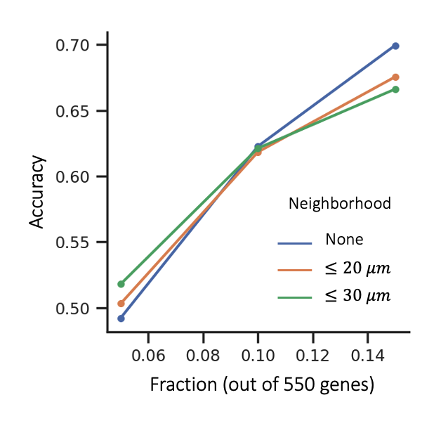
We found that gene expression in neighboring cells can improve supertype classification when fewer genes are available.
Node embeddings
Having found that neighboorhood information can be helpful for cell type classification, we wanted to see if the neighborhood structure of a cell by itself (without any gene expression information) can be informative of cell types. To do so, we use node embedding methods.
Node2Vec learns an embedding \(f(u)\) that is predictive of the neighborhood \(\mathcal{N}(u)\) of each node \(u\).
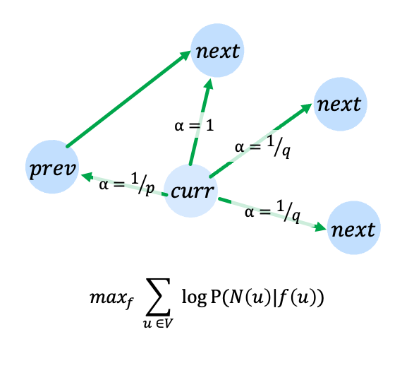
The neighborhood for each node is determined through fixed length, 2nd order random walks starting from each node. Parameters \(p\) and \(q\) determine the transition probabilities for the random walk.
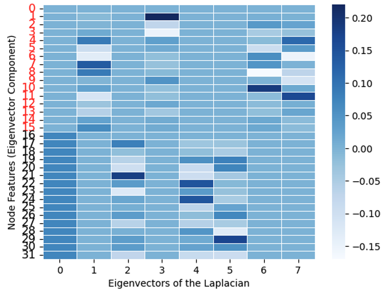
Spectral graph clustering frames the problem as an eigen decomposition (Von Luxburg 2007).
Specifically, the eigenvectors of the Laplacian matrix are used as features for clustering.
Simulation
We build intuition for how embeddings based on peptidergic connectivity could partition cells into meaningful groups even in the absence of explicit gene expression information with a toy problem.

We start with a type x type adjaceny matrix that shows which cell types can communicate with which cell types. The type x type adjacency matrix can be sampled to obtain a cell x cell adjacency matrix. The block structure is equivalent to the graph having distinct connected components (as shown on the right).
Code for Node2Vec and spectral graph clustering applied to the simulation can be found here.
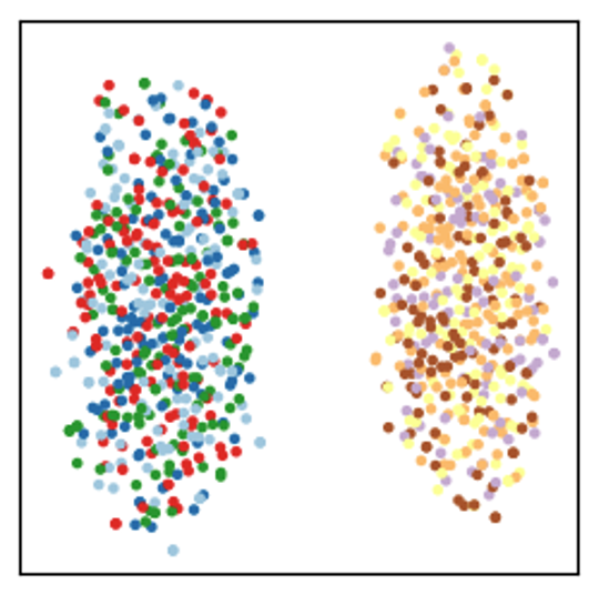
Clustering the embeddings obtained with Node2Vec is a scalable way to identify such components. We found that spectral graph clustering can identify these components too. However, spectral graph clustering has limited applicability to our dataset given its computational complexity of \(O(n^3)\) (Von Luxburg 2007).
Conencting this back to the problem of peptidergic communication, we can think of the dark blue, light blue, red, and green nodes as 4 cell types that communicate with each other, and the yellow, brown, orange, and violet nodes as 4 cell types that communicate with each other. This type x type adjacency matrix denotes 1 communication network between the cells or 1 layer in the multilayer graph. With 1 layer, we can distinguish between 2 groups of cells.
Multilayer graph clustering
For multilayer graphs, one approach to obtain embeddings for the whole graph is to obtain independent embeddings for each layer in the multigraph. Combining information from each embedding can identify all the ‘types’ when the blocks are chosen carefully across layers.
If we have n types \((t_1,…,t_n)\) and k layers \((X_1,…, X_k)\):
\(P(t_i) = \frac{1}{n}\)
\(P(t_i | X_1) = \frac{2}{n}\)
\(P(t_i | X_1, X_2) = \frac{4}{n}\)
\(P(t_i | X_1, X_2, ..., X_k) = 1\)
where \(k = \log_2 n\)

An embedding is generated from each type x type matrix. The 3 embeddings are concatenated and visualized with TSNE. We see that with 3 layers, we can perfectly distinguish between the 8 cell types. Simiarly, we hypothesize that with 3 peptidergic communication networks, we can distinguish between 8 groups of cells.
Node2Vec performance against noise/sparsity
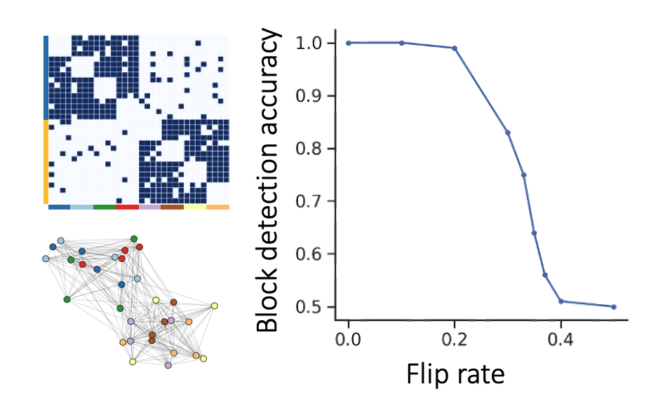
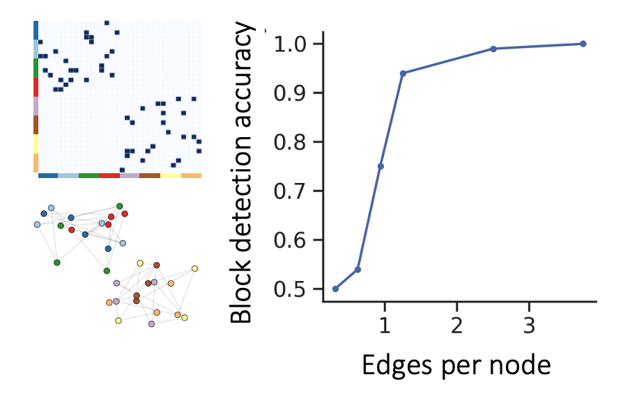
Because gene expression data is noisy and our peptidergic communication networks are quite sparse, we study Node2Vec’s performance when faced with these issues. We see that Node2Vec embeddings cluster according to the underlying block structure in a manner that is robust to sparsity as well as noise in the cell x cell graph.
| Noise experiment | Sparsity experiment |
|---|---|
 |
 |
Application to MERFISH VISp data
We apply Node2Vec to MERFISH VISp data to inspect the utility of graph embeddings in identifying celltypes (subclass) and spatial groupings.
We consider 4 different methods of obtaining Node2Vec embeddings.
- considering only proximity of cells in the graph (distance)
- concatenating embeddings of individual peptidergic graphs (independent)
- collapsing the multi-layer graphs into a single layer graph (squashed)
- jointly considering the multilayer graphs with an adapted Node2Vec model (joint)
For the joint method, we sample random walks from all layers to determine the neighborhood for each node (as opposed to neighborhoods constructed from only 1 layer). To do so, we modify the Pytorch Geometric implementation of Node2Vec.
Code for distance, independent, squashed, and joint.
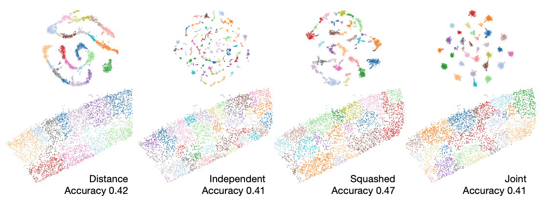
We observe that even in the absence of explicit gene expression information, embeddings obtained from peptidergic connectivity contain information about cell types. We speculate that cell clusters obtained with leiden clustering correspond to spatial domains relevant from a functional point of view.
Gene Imputation
We speculated that with more communication channels (more layers in the peptidergic multilayer graph), we should be able to distinguish between cells with higher accuracy (only 5 communication channels were available in the dataset out of 37 putative channels). To test this hypothesis, we tried gene imputation methods. Gene imputation methods can be used to recover the expression of peptidergic communication genes that were not part of the MERFISH dataset. Several tools have been benchmarked for this task (Li et al. 2022), and we used the top performing model Tangram to impute values of all peptidergic communication genes.
Tangram maps cells from a scRNA-seq dataset to cells (or voxels) from a spatial transcriptomic dataset (Biancalani et al. 2021). Tangram learns a mapping matrix M defined such that \(M_{ij} \geq 0\) is the probability of cell i (from scRNA-seq) mapping to cell \(j\) (from spatial transcriptomic data). The loss function used to optimize M is shown below.
\[ L(S, M) = \sum_{k}^{n_{genes}} \cos_{sim} ((M^T S)_{*, k}, G_{*,k}) \]
S: scRNA-seq matrix (cell x gene)
G: spatial transcriptomic data matrix (cell x gene)
M: mapping matrix (cell * cell)
We assessed imputation performance by using peptidergic communication genes that were already measured as test data.
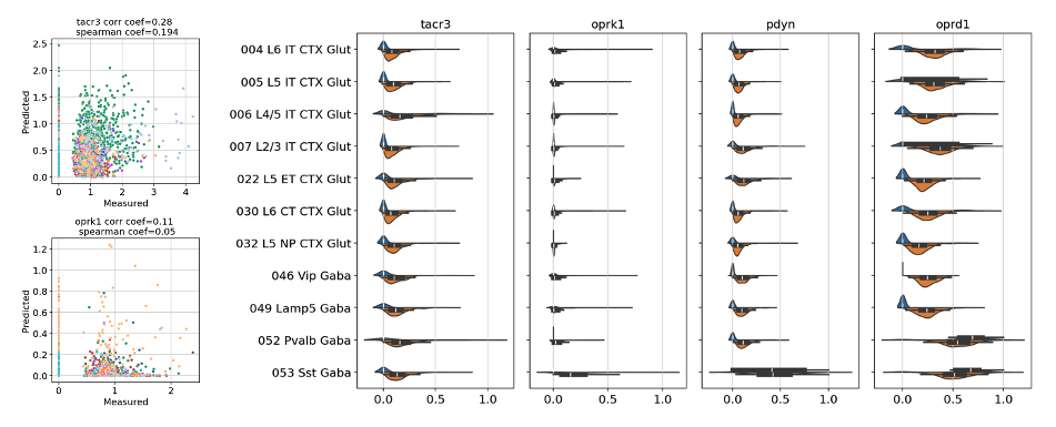
We found that the correlation between imputed gene expression and actual gene expression is not strong enough for us to use imputed results in our multilayer graphs. In particular, a non trivial amount of null gene expression values were mapped to positive values.
Limitations and future work
Only 5 out of the 37 cognate neuropeptide precursor and GPCR pairs were experimentally measured in the MERFISH dataset, which precludes an assessment at more detailed levels of the taxonomy. Neuron morphology may be an important consideration relevant for the full spatial extent of peptidergic communication. Arbor density representations derived from patch-seq datasets could offer a way forward.
The poster can be found here.
Code repository: https://github.com/donghyunkm/cciGraphs
We thank Tom Chartrand, Ian Convy, Olga Gliko, Anna Grim, Yeganeh Marghi, Uygar Sümbül, Meghan Turner, and Kasey Zhang for helpful feedback and discussions.